ml5.js Classification and Regression Analysis

GitHub Repository: https://github.com/Ashot72/ml5-spfx-extension

Video link: https://youtu.be/NbO_ZIVHdus

ml5.js https://ml5js.org/ aims to make machine learning approachable for a broad audience of artists, creative coders, and students. The library provides access to machine learning

algorithms and models in the browser, building on top of TensorFlow.js with no other external dependencies.

I built an ml5 SPFx extension for classification and regression analysis. I already built a KNN app (k-nearest-neighbor algorithm, machine learning algorithm)

https://github.com/Ashot72/knn-tensorflowjs-spfx-extension for classification and regression analysis using TensorFlow.js  https://www.tensorflow.org/js.

You may read KNN first as I described how to import .csv data into SharePoint lists, displayed some of TensorFlow.js operations, normalization, talked about

features and labels which are also present in this app.

Actually, there are 2 sets of TensorFlow APIs. First one is low level linear algebra API that I used in KNN app and the second one is higher level API that makes

pretty easy to make some more advanced machine learning algorithms. We use ml5.js which was built on top of the TensorFlow.js which makes even much easier to

work with tensorflow.js.

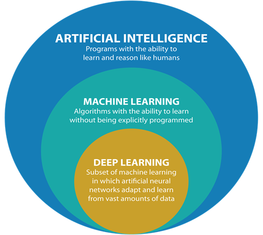
Figure 1

Deep Learning is a subset of machine learning in which artificial neural networks adapt and learn from vast amounts of data. With tensorflow.js you can build a neural network with the

help of layers and model.

Model is a data structure that consists of layers and defines inputs and outputs.

In the context of neural networks, a layer is a transformation of the data representation. It behaves like a mathematical function: given an input, it emits an output. A layer can have

state captured by its weights. The weights can be altered during the training of the neural network. Usually we do not define layers with ml5.js though it is possible.

Before running analysis, we should understand if we solve classification or regression problem.

A classification problem has a discrete value as its output. It is not necessary to have 0/1 or true/false output in classification case. The output can for example be colors such as,

red, green, blue, yellow etc. some discrete values.

A regression problem does not deal with discrete values. For example, to find a price of a house based on its location, bedroom etc. Price is a continues value. It can be $20000 or $200001 etc.

Multi linear Regression Analysis

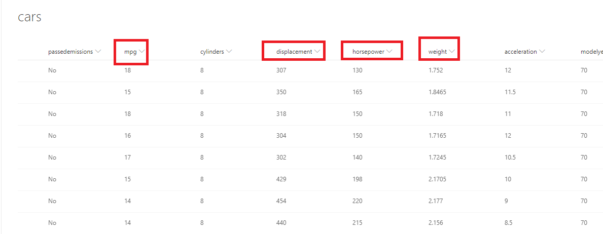
Figure 2

This is our cars SharePoint list.

Mpg - miles per gallon is the efficiency of the car telling you how many miles it can travel or how much distance it can travel per gallon.

Displacement - more or less is the size of the engine.

Horsepower - the power of the engine.

We are going to figure out some relationship between some dependent variables and independent variables using a linear regression approach. With linear regression we are going to do

some initial training of our model which takes some amount of time (seconds, minutes, hours depending of the size of the dataset). Once we have the model that has

been trained, we can then use it to make a prediction very quickly.

So, what is the goal of linear regression?

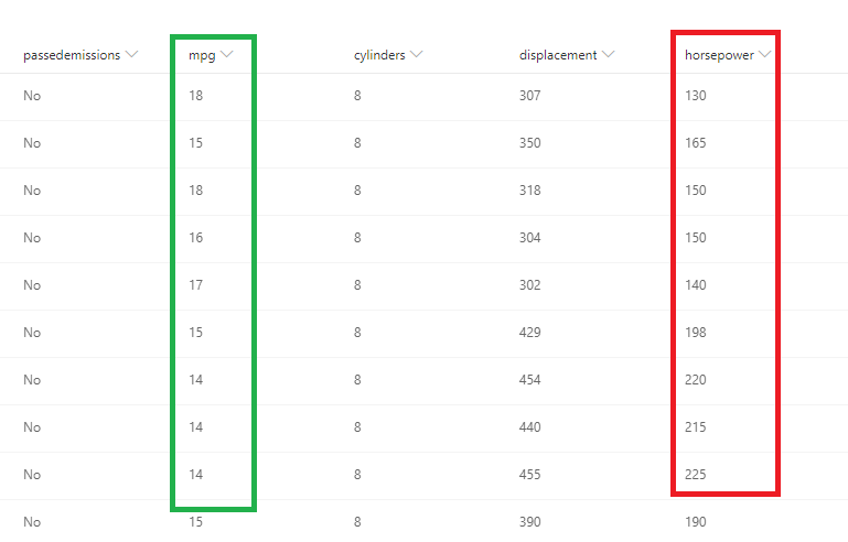
Figure 3

We are going to find an equation to relate some independent variable to a variable that we are going to predict usually referred as the dependent variable. In this case we might try to figure out some type of

mathematical equation; for some particular horsepower value we predict mpg (miles per gallon). We are going to have some input data and use some algorithm to predict some output data.

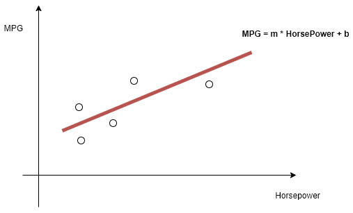
Figure 4

The goal of linear regression is to predict a relationship between those variables which takes the form of an equation like MPG = m * HorsePower + b (e.g. MPG = 200 * HorsePower + 20).

We should figure out m and b. m is the slope of the line and b is the bias. This equation is represented by a line that might be used to kind of predict or fit between all of our different data points.

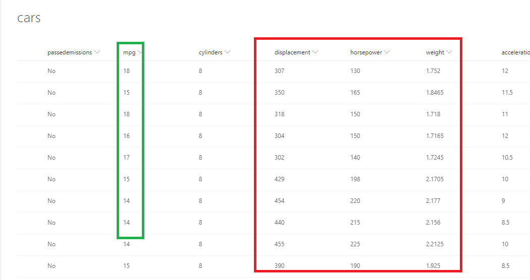
Figure 5

With linear regression we are not restricting to having just one independent variable. We can very easily have multiple independent variables.

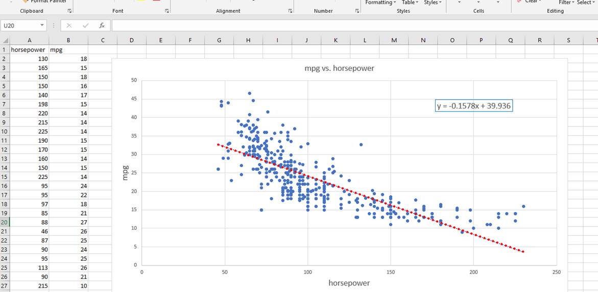
Figure 6

I did linear regression analysis using Excel scatterplot chart. I plotted out some independent variable (horsepower) and dependent variable (mpg) and found some mathematical relation

between two y = -0.1578x + 39.936.

Before going ahead, I would like to tell you just a few words about Residual analysis. The analysis of residuals plays important role in validating the regression model.

Residual refers to the difference between observed value vs. predicted value and every data point has one residual.

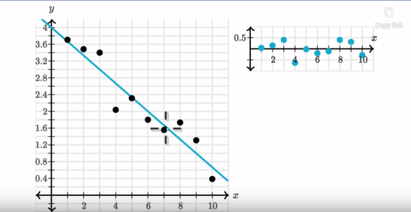
Figure 7

Right here we have a regression line and its corresponding residual plot (you can produce a residual plot in Excel).

It looks like these residuals are pretty evenly scattered above and below the line. We could say that a linear model here, the regression line, is a good model for this data.

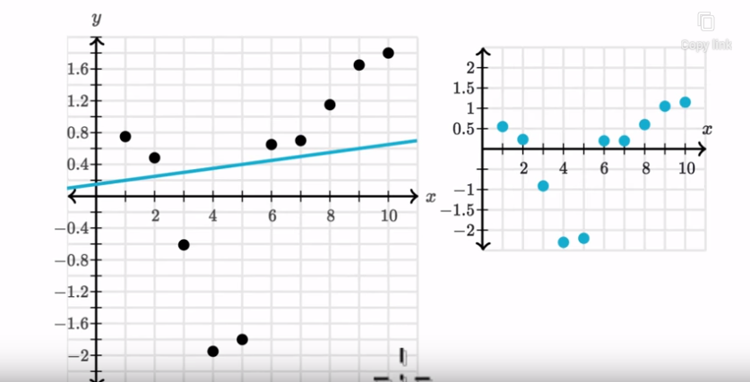
Figure 8

When you look at just the residual plot, it does not look like they are evenly scattered. It looks like there is some type of trend here.

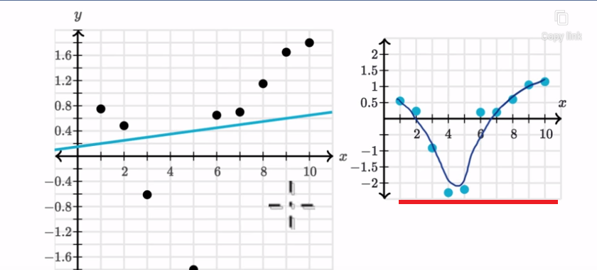
Figure 9

Where you see something like this, where on the residual plot you are going below x-axis and then above then the linear model might not be appropriate. Maybe some type of non-linear model.

Some type of non-linear curve might better fit the data and the relationships between y and x are nonlinear.

How to solve a linear regression problem?

There are many different approaches to solve linear regression problems; Ordinary Least squares, Generalized Least Squares, Gradient Descend etc. Gradient Descent

is an approach that is used in many other very complicated machine learning algorithms. I do not want to go into the details as there are tons of articles about it but in general

Gradient Descend is a general function for minimizing a function, in regression case, the Mean Squared Error cost function.

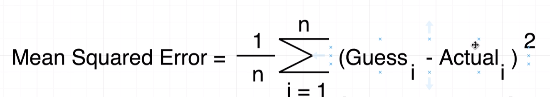
Figure 10

Means squared equation (MSE) essentially produces a value that tells you how wrong or how bad your guess is. It basically tells you how close a regression line is to a set of points.

It does this by the distances from the points to the regression line (these distances are the 'errors') and squaring them. The squaring is necessary to remove any negative signs.

It also gives more weight to larger differences. It is called mean squared error as you are finding the average of a set of errors. (Guess - Actual can be Actual - Guess as it is squared).

Σ summation symbol means take every one of your guesses and every one of your actual values find the difference between the two, square the result and then

some them altogether.

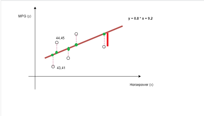
Figure 11

Let's imagine that some actual values are (43,41), (44,45) etc., the green ones are guessed values and the equation is 0.8 * x + 9.2. Guess - Actual is essentially the

dotted line distance, the 'error'. Let's calculate MSE for the following set of actual values: (43,41), (44,45), (45,49), (46,47), (47,44)

Find the guesses based on y = 0.8 * x + 9,2 equation.

0.8 * 43 + 9.2 = 43.6

0.8 * 44 + 9.2 = 44.4

0.8 * 45 + 9.2 = 45.2

0.8 * 46 + 9.2 = 46.8

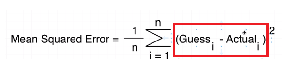
Figure 12

Now, calculating Actual - Guess (calculating Actual - Guess instead of Guess - Actual as it should be squared at the next step).

41 - 43.6 = -2.6

45 - 44.4 = 0.6

49 - 45.2 = 3.8

47 - 46 = 1

44 - 46.8 = -2.8

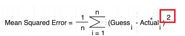
Figure 13

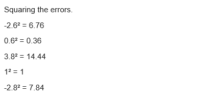
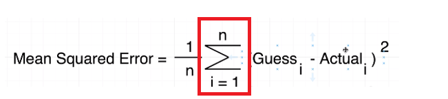
Figure 14

Add all of the squared errors up: 6.76 + 0.36 + 14.44 + 1 + 7.84 = 30.4

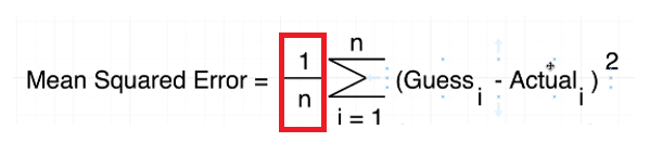
Figure 15

Find the mean square error 30.4 / 5 = 6.08

You might be curious, 6.08 what? What is that number actually mean. MSE in isolation is not actually that useful. We can not actually look at this number

and say that it is a good guess or this is a bad guess. In order to quantify this guess and say that 6.08 is good or bad guess we have to run the MSE again

with some other guess. We have to come up with a new equation for the relationship between X and Y variables and run that equation again.

Once we have the second value for MSE we can say whether or not 6.08 was good. In other words, MSE is only producing a value that we can compare

in relation to other values to say whether or not a particular guess is good or bad.

For the first y = 0.8 * x + 9,2 equation MSE is 6.08. Just imagine for another equation y = -1.8 * x - 20,2 MSE is 4.2.

MSE 4.2 is smaller than 6.08 then we are closer the line of best fit.

You must be thinking that if we could ever get our MSE down to zero then we must have like a perfect guess. Even if we come up with an extremely good guess

(Figure 11, it looks like it is probably as good a guess as we could possibly get with a straight line) there is still some distances in there (the dotted lines).

MSE is unlikely to ever be exactly zero. If we could find a very low value of MSE we would have a very good equation or a very good guess.

Natural Binary Classification - Logistic Regression

With linear regression we are prediction continues values. For example, given the horsepower of a vehicle we predict its mile per gallon (mpg) value which can be 13,24, 45 etc.

With logistic regression we are going to use the algorithm to predict discrete values. Logistic regression is used for classification type problems. Binary classification problem is when we

take an observation and then put it into one of two categories. For example, given some users age are they likely to prefer an Apple phone or an Android phone. Either A or B option, no other options.

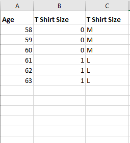
Figure 16

Here is the problem we want to solve. Given a person's age, do they wear M T Shirt or L? Note, we have just one feature Age, and there are only two possible label values that we

could apply to a single person; a person either wears M shirt or L. This means this is a binary classification problem.

Our goal is to find a mathematical relationship (a formula) that relates a person's age to whether they like to wear an M shirt or L shirt.

We have a dataset of 6 items. Let's assume that people from age of 58 - 60 wear M shirt while people over 60 wear L size, just an assumption.

In preferred size = m * age + b formula, preferred size should be a number and for that reason we replace M with 0 and L with 1 as there is no way to

multiply a number by the string M or L.

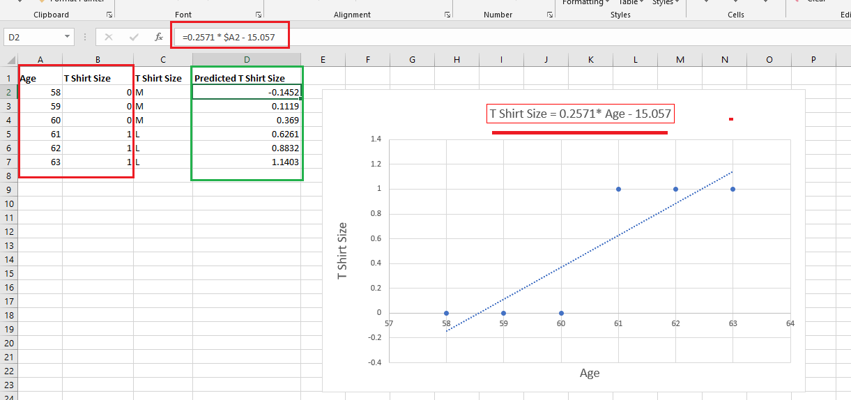
Figure 17

I did linear regression analysis with the independent variable Age, and dependent variable T Shirt Size and plotted it out in Microsoft Excel.

The equation is y = 0.2571 * x - 15.057 where x is the Age. You may notice that someone who is 58 years old was predicted to have T Shirt Size value of -0.1452.

Someone who is 63 was predicted to have a T Shirt Size value of 1.1403. In some cases, we have values greater than one (1.1403), in some cases we got predicted values that are

negative (-0.1452). In some other locations we got values that are between 0 and 1 such as 0.369.

Let's assume for a moment that predicted values between (0 - 1) are OK, outside (0 -1) are not good results. It has no meaning to us. The thing is that if we use an equation m*x + b we

will never be able satisfy the requirement and predicted values should be inside 0 -1 range. We need to find out some other equation that is going somehow to give us a relationship

between Age and our predicted T Shirt Size that is not of the form of m *x + b.

Figure 18

We are going to guess a different value of m and b by putting different x values to this equation. e in this equation is Euler's constant number that is approximately equal to 2.718

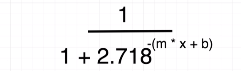
Figure 19

The equation looks like this if you replace e with 2.718 in the formula.

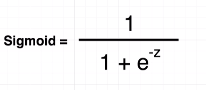
Figure 20

General form of this equation is what we call sigmoid equation which always produces a value between 0 and 1. It really fits our problem when we were saying that only values between 0 and 1

give us some meaningful output.

Figure 21

If we plug in some value of z right in the formula (Figure 20), what we are always going to get out is some value that ranges from 0 to positive 1.

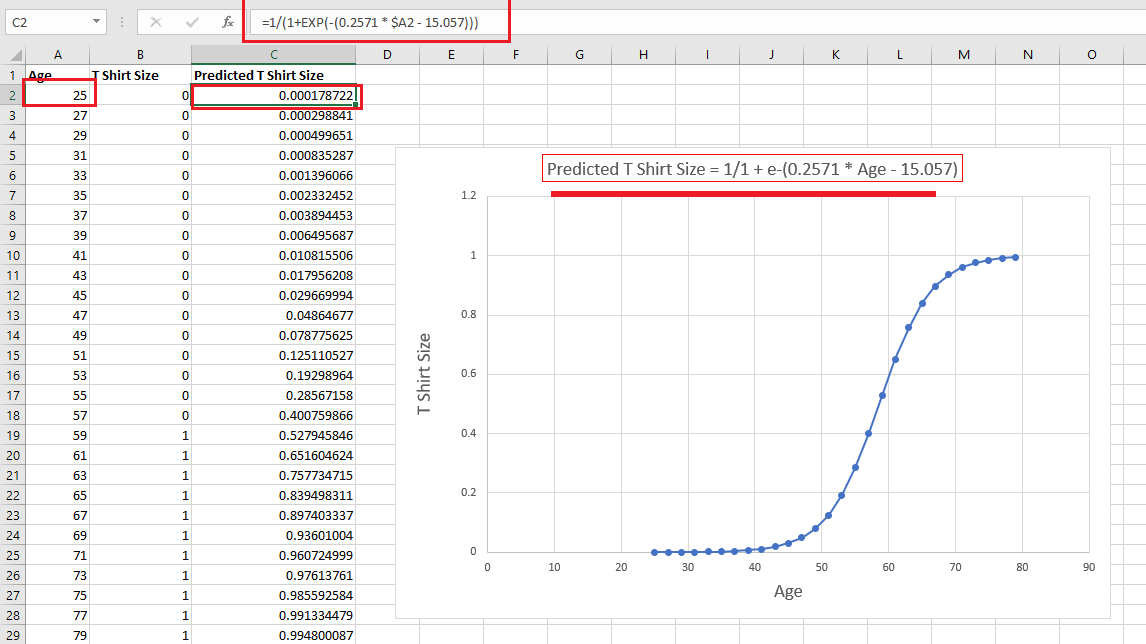
Figure 22

With our sigmoid equation I plugged in different values of ages and got predicted T Shirt Size. You see that this time predicted values are between 0 and positive 1. For the predicted value of age 25 I got

0.000178722 which is close to zero which indicates that someone with the age of 25 will wear M Shirt Size.

Let's understand a little bit more why we only care about values coming out of that equation that range between 0 and 1.

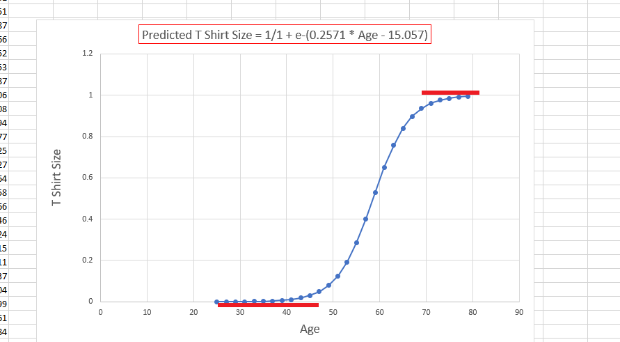
Figure 23

The closer the line gets down to zero the more likely that someone will wear M Shirt and as the line gets closer to one it is more likely that someone wears S Shirt.

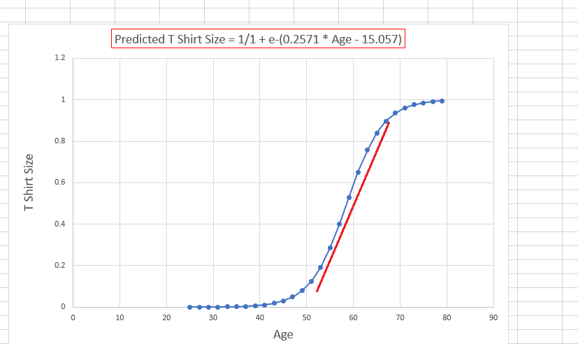
Figure 24

There is an area where the line crosses over from 0 to 1 and it is a relatively gradual shift.

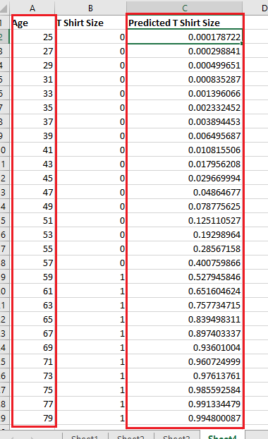
Figure 26

People started with predicted value very close to zero which means they are likely to wear M shirt then as they are getting older

57, 59 etc. years old people then the predicted values are 0.40, 0.52 etc. which means a gradual shift; wanting to wear L shirt. What the values

that are not close to zero or one really mean for us? The output of sigmoid equation in this example is probability of someone wearing L shirt.

Now, we can say someone who is 25 years old has a probability of 0.000178722 (or 0.0178722 percent) of wearing L shirt. No chance to wear L shirt.

When someone is getting 51 years old their probability of wearing L shirt is 12.51 percent.

The point of the logistic regression is not to get a probability but care about classification. We should just say these people wear M shirt and those ones L shirt.

We should say that with a probability less than this amount is going to be assigned to label zero otherwise to one.

We refer to that as decision boundary.

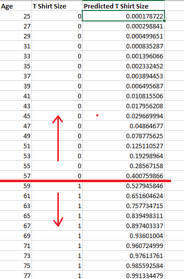
Figure 27

A common decision boundary to use would be .5. This mean that people with a probability of greater than 0.5 will be assigned to one label classification and the others to zero.

For some problems the decision boundary may not be 0.5 say .99 might make a lot of sense. An example of this can be safety analysis, cause a threat to human life

versus not to cause a threat to human life. You want to make sure you are not causing threat to human life 99% of the time.

Multi-Value Classification - Multinomial Logistic Regression

With multinomial logistic regression we have the ability to apply multiple different label values to classify a given observation. For example, given a person's age what type of phone

do they prefer - Android, Apple or Windows phone. There is no single either or (e.g. Android or Apple) it might be the wide range of phones. So, a binary classification problem could be

turned into multiple classification type of problem with additional options or label values.

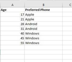
Figure 28

This is a dataset similar to what we already have for binary classification (age, shirt). People ages and their preferred phones.

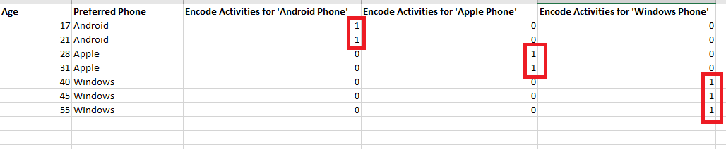
Figure 29

We are going to encode the values differently. We are going to do it three separate times and take a look at all the different possible classification values. There are three distinct possible

label values Android phones, Apple phones and Windows phones. We use all these encoded values to produce a new different encoded label set.

This type of encoding is called one hot encoding which is a process by which categorial variables are converted into a form that could be provided to

Machine Learning algorithms to do a better job in prediction.

Marginal vs Conditional Probability

Marginal Probability Distribution is when we have probabilities that considers each possible output case in isolation.

Conditional Probability Distribution is going to consider all possible output cases together when putting together a probability.

We are calculating Marginal Probability Distribution when we make use of Sigmoid function.

Suppose we do our analysis with different data set and we get as a result a .35 probability for someone using Android Phone, .30 for Apple and .40 for Windows Phone.

We will take the highest probability .45 and could say that this person uses Windows Phone.

Figure 30

What those probabilities are telling us in terms of sigmoid function?

Probability values that we see are probabilities of some observation using, say, .35 percent Android phone but it is no claiming about this person's probability

of using Apple or Windows phones.

With a marginal probability distribution, we get these probabilities that are only informing the probability of a single output; a single characteristic.

In general, it is possible that someone is using both Android, Apple and Windows phone but in the classification analysis we do not really want to see a person

capable of doing across a wide spectrum. We do not care that someone wants use an Android phone, Apple or Windows. We only care about the phone

that he is most likely going to use. We do not want a marginal probability distribution for these probabilities we are calculating, because a marginal distribution

is going to essentially give us probabilities of just a single outcome in isolation; just using Android phone, just using Apple phone, just using Windows phone.

When you are working with marginal probability distribution you can sum all these probabilities together.

.30 + .40 + .45 = 1.15

If you sum these probabilities and see that the total is not just up to 1 then it possible means you are working with a marginal probability distribution.

Now, just imagine that a probability of using Android phone is 0.3, Apple is 0.5 and Windows is 0.2.

0.3 + 0.5 + 0.2 = 1

This possibly means we are working with a conditional probability distribution as the sum is up to 1, and there is some interconnected meaning with each other.

Sigmoid vs Softmax

Sigmoid equation is always going to result in a marginal probability distribution. If we want to move over to get into a conditional all we have to do is use a slightly different equation.

Instead of Sigmoid we are going to move over to a different equation called the Softmax equation. The Softmax equation is specifically written to essentially consider different output classes

and give us probabilities that kind of do not isolate one output by itself. Instead, it is going to take a couple of different probabilities and relate them (in relation of each other).

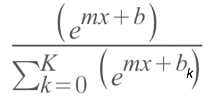
Figure 31

On the denominator we are going to take mx + b value of all our different classifications and sum them all together.

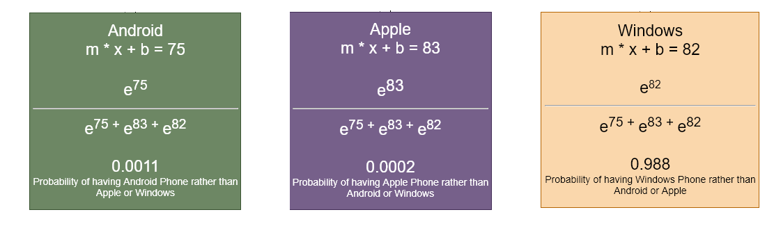
Figure 32

For using Android phone, we have an equation mx + b = 75. We are taking mx + b values and put them into the equation (Figure 31). With this Softmax equation we are considering

all the other possible outcomes because it uses the outputs of those different classification values.

If we total up the probabilities it should be just 1.

0.0011 + 0.0002 + 0.988 = 1

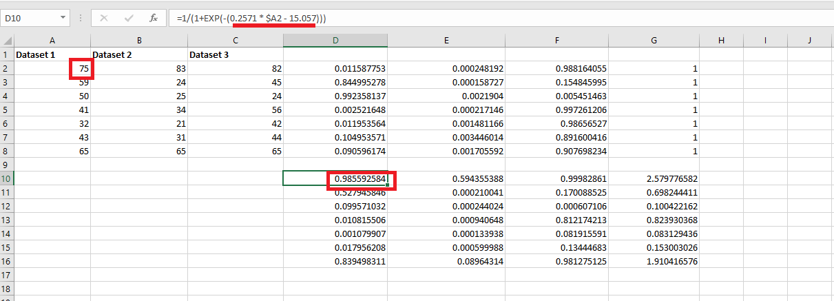
Figure 33

I would like to show the difference between Sigmoid and Softmax in Excel.

You see sigmoid function (Figure 30) in the formula bar. For Dataset 1, mx + b part is 0.2571 * $A2 - 15.057 where $A2 is the absolute cell reference.

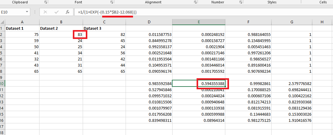
Figure 34

For Dataset 2 we assigned different values for m and b in mx + b equation and another one is assigned for Dataset 3.

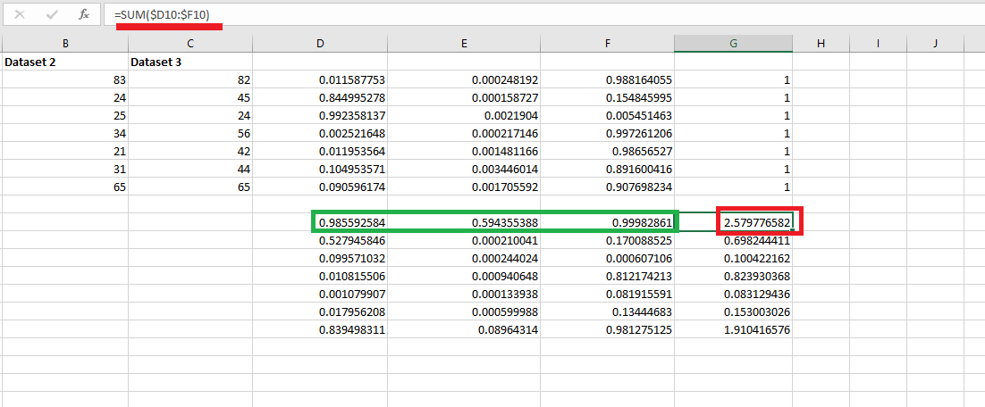
Figure 35

The sum of those three probabilities is not 1.

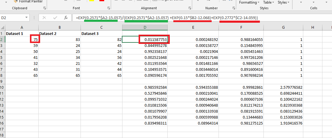
Figure 36

We have the same mx + b equation this time plugged into Softmax equation (Figure 31).

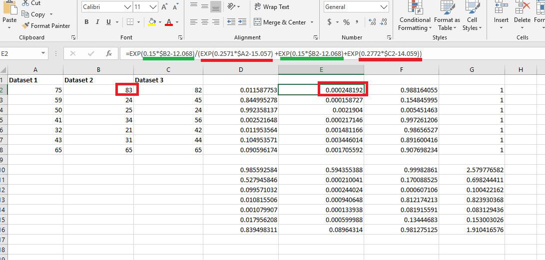
Figure 37

For Dataset 2.

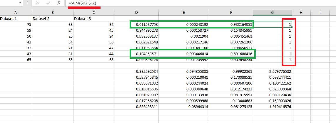
Figure 38

The sum is always 1.

Neural Networks

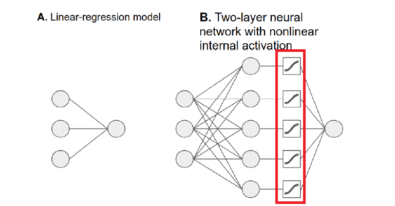
Figure 39

Machine learning is a huge topic and it is simply not possible to cover everything.

Option A illustrates a linear regression model. Option B is a reduced two-layer network and the difference is that option B illustrates the nonlinear

(e.g. sigmoid that you already know) activation function.

Activation functions are mathematical equations that determine the output of a neural network and used at the last stage of a neural network layer. Activation function can be linear

and nonlinear. Nonlinear activation functions can be used to increase the representation power of a neural network. Examples of nonlinear activations include sigmoid, hyperbolic

tangent (tanh) as well as the rectified linear unit (ReLU) function.

The sigmoid function is a squashing nonlinearity, in the sense that it squashes all real values from -Infinity to +Infinity into a much smaller range -1 to 1.

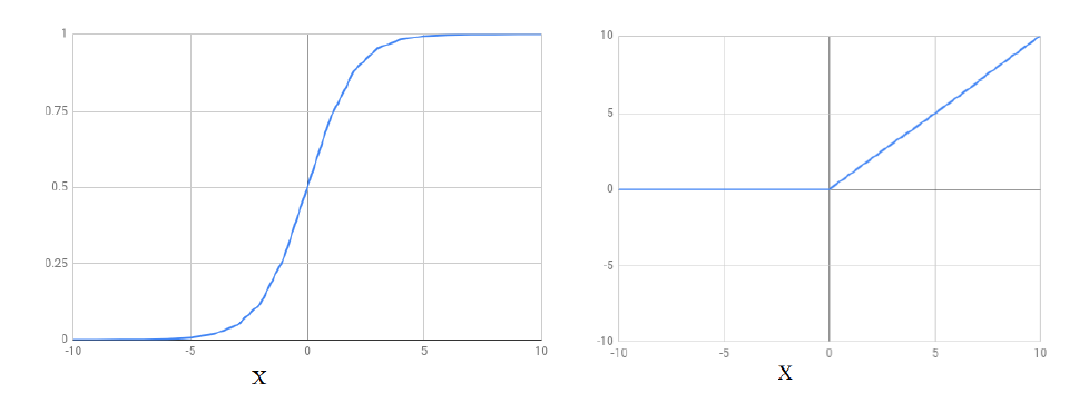
Figure 40

On the left it is the sigmoid function S(x) = 1 / (1 + e ^ -x) and on the right it is relu function relu(x) = { 0: x< 0,x: x>= 0}

How nonlinearity improves the accuracy of the model? Many relations in the world are linear. For example, a linear relationship between production hours and output in a factory

means that a 10 percent increase or decrease in hours will result in 10 percent increase or decrease in the output. Many others are not linear; relation between a person's height

and his/ger age. The height varies roughly linearly with age only up to a certain point. A purely linear model cannot accurately model height/age relation, while the sigmoid

nonlinearity is much better suites to model relation. In order to prove it you can create a, say, 2 layered model in tensorflow.js and run the app with a sigmoid activation function

or without it (just comment activation: 'sigmoid' line). You will see that the one without sigmoid activation leads to higher final loss values on the training.

Another question you may ask is by replacing a linear activation with a nonlinear one like sigmoid, do we lose the ability to learn any linear relations that might be present in the data?

The answer is no.

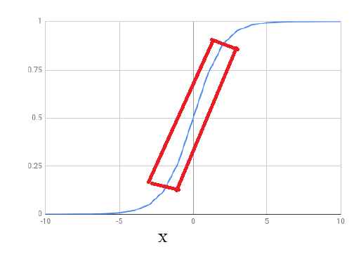
Figure 41

The part of the sigmoid function (the part closer to the center) is fairly close to being a straight line. Other frequently used nonlinear activation functions such as tanh and relu

also contain linear or close to linear parts. If the relation between certain elements of the input and output are approximately linear, it is entirely possible for a layer with a nonlinear

activation to learn the proper weights and biases to utilize the nonlinear part of the activation function.

Another important thing to understand is that nonlinear functions are different from linear ones is that passing the output of one function as the input to another

function (cascading) leads to richer sets of nonlinear functions.

Let's see it in action.

Figure 42

Navigate to https://www.wolframalpha.com/

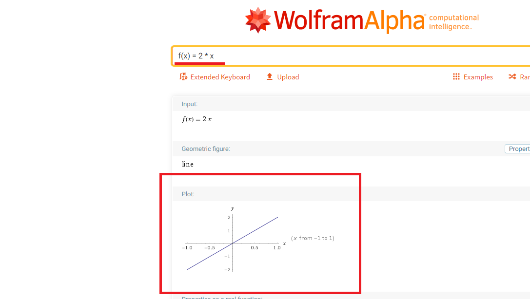
Figure 43

Input f(x) = 2 * x linear function to see the plot.

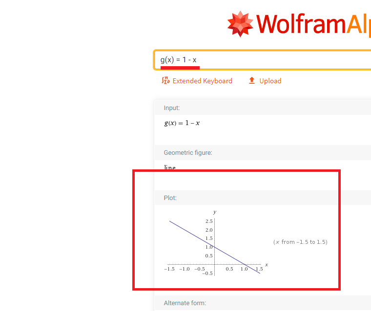
Figure 44

g(x) = 1 - x is the second function.

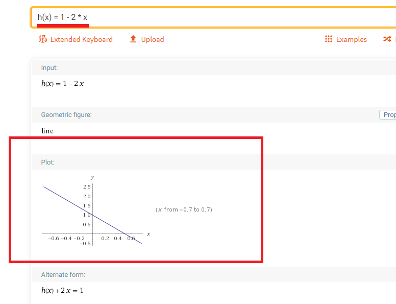
Figure 45

Let's cascade these two functions to define a new function.

First function is f(x) = 2 * x, the second one is g(x) = 1 - x

New, h(x) = g(f(x)) = 1 - 2 * x

As you can see, h is still a linear function. It just has a different slope and bias. Cascading any number of linear functions always results in a linear function.

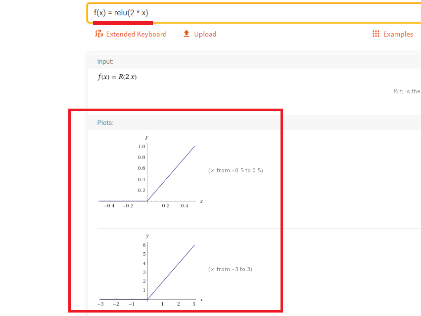
Figure 46

Now, cascading two nonlinear relu functions.

The first function is f(x) = relu(2 * x)

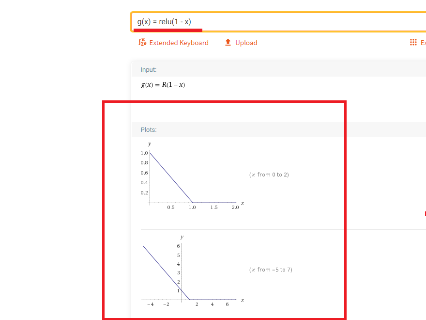
Figure 47

The second one is g(x) = relu(1 - x)

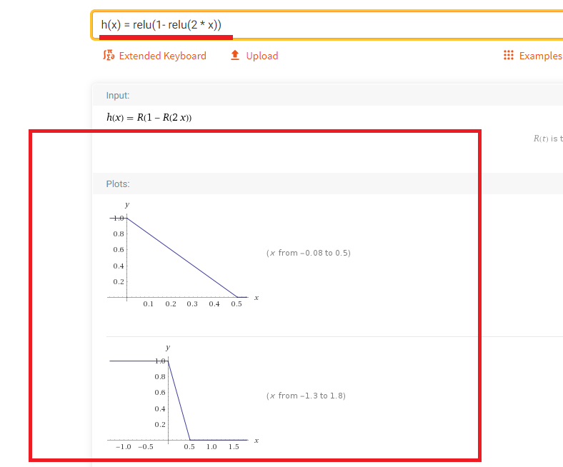
Figure 48

First function is f(x) = relu(2 * x), the second one is g(x) = relu(1 - x)

New, h(x) = g(f(x)) = relu(1- relu(2 * x))

By cascading two scaled relu functions, we get a function that does not look like relu at all. It has a new shape. Further cascading the step function with other relu functions

will give you more diverse set of functions. In essence, neural networks are cascading functions. Each layer of a neural network can be viewed as a function. Nonlinear activation

functions increase the range of input-output relations the model is capable of learning.

Application

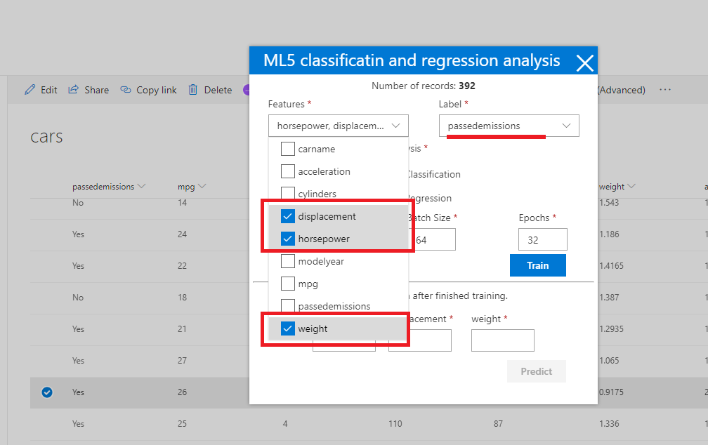
Figure 49

We select three features displacement, horsepower and weight and passedemissions as the label.

Given a vehicle's weight, horsepower, and engine displacement, will it PASS or NOT PASS a smog emissions check?

That is the problem we should solve.

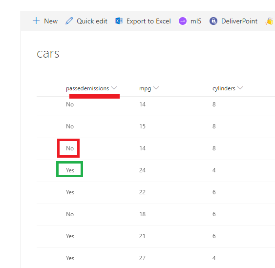
Figure 50

Notice, here for smog emissions we have two possible label values. It is definitely a binary classification problem.

A given car can either pass or not pass a smog emissions check.

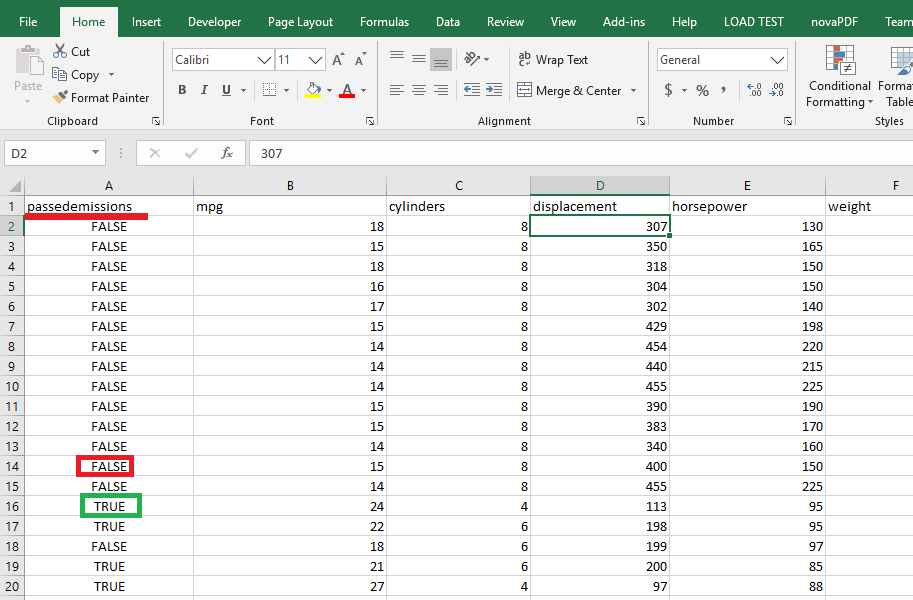
Figure 51

SharePoint Cars list has been imported from cars.csv file and SharePoint convert a true/false value to Yes/No.

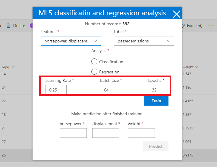
Figure 52

You may notice that there are some options we specified which requires for training. These are called hyperparameters.

Hyperparameters - are adjustable parameters in the model that must tuned in order to obtain a model with optimal performance

(lowest validation loss after training). The process of selecting good hyperparameter values is referred to as hyperparameter optimization or

hyperparameter tuning. Unfortunately, there is currently no definitive algorithm that can determine the best hyperparameters given a dataset and

the machine-learning task involved.

Learning rate - is a hyperparameter that controls how much to change the model in response to the estimated error each time the model weights are updated.

Choosing the learning rate is challenging as a value too small may result in a long training process that could get stuck, whereas a value too large may result in

learning a sub-optimal set of weights too fast or an unstable learning process. The learning rate may be the most important hyperparameter when configuring

your neural network.

Batch size - hyperparameter defines the number of samples that will be propagated through the network. The higher the batch size, the more memory space

you will need.

Epochs - One epoch is when an entire dataset is passed both forward and backward through the neural network only once

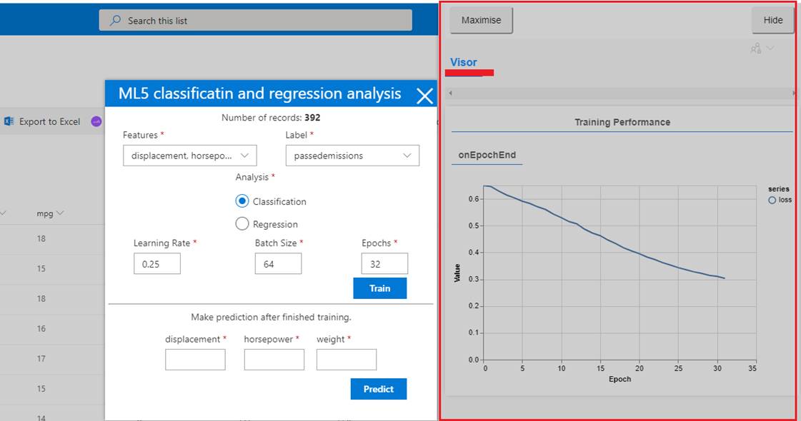
Figure 53

Once you click the train button you will see loss vs epochs plot.

A loss function is an error measurement. This is how network measures its performance on the training data and steers itself in the right direction. Lower loss is better. As we train,

we should be able to plot the loss over time and see it going down. If our model trains for a long while and the loss is not decreasing, it could mean that our model is not learning to

fit the data.

The loss function that we use for binary classification task is binary cross entropy, which corresponds to the binaryCrossEntropy configuration in the model.

Our problem is a binary classification problem as we stated. Vehicles will either PASS or NOT PASS a smog emissions check.

The configuration in multiclass or multinomial classification case is the categoricalCrossentropy which categorizes data points more than two options (blue, green, yellow).

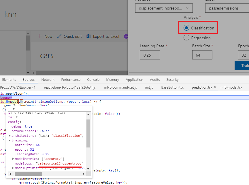
Figure 54

ml5.js prefers categoricalCrossentropy option for modelLoss instead of binaryCrossEntropy one for our binary classification problem.

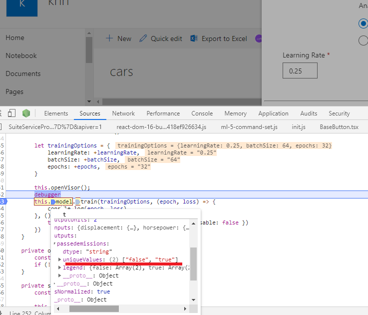
Figure 55

It knows that there are 2 options but categoricalCrossentropy is the choice anyway.

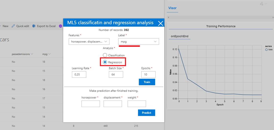
Figure 56

Given a vehicle's weight, horsepower, and engine displacement, we want to predict mile per gallon mpg value. It is a multilinear regression problem.

A regression problem does not deal with discrete values as the mpg here can be 13, 14, 25 etc.

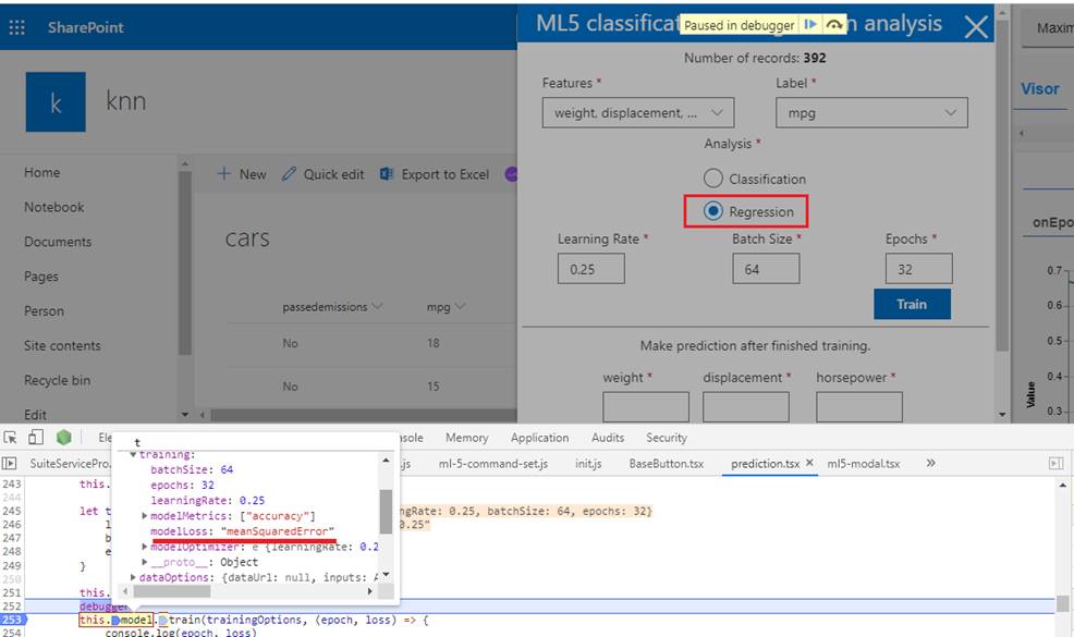
Figure 57

For the regression case the modelLoss is set to meanSquaredError which we already discussed.

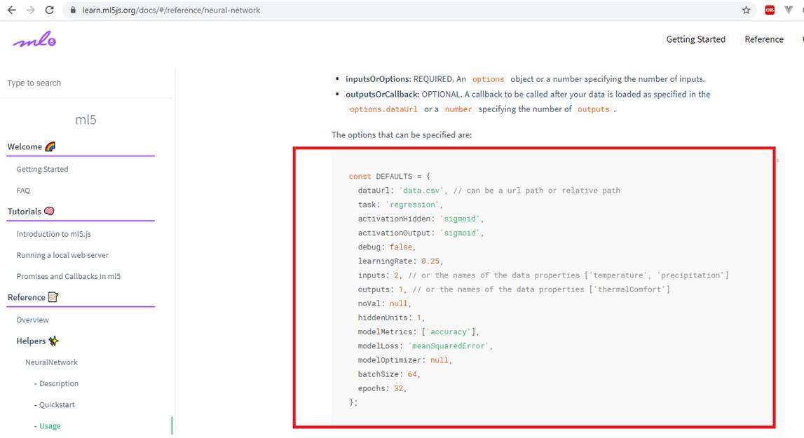
Figure 58

If you navigate to ml5 web site you will see some default options that is required for neural networks. You can modify them which we already did for learning rate, batch size and epochs.